Parallel Graph Search (A Case Study)An in-depth analysis of common graph search algorithms such as Bellman-Ford, Dijkstra and A-star and their parallelized counterparts. |
|
TL;DRThis article does an in-depth analysis of three major graph search algorithms: Bellman-Ford, Dijkstra and A-star algorithms and explores ways to parallelize them. The article first goes through the theoretical analysis of each of the algorithms and then shifts onto practical analysis confirming the predictions of theoretical analysis on GPUs: Nvidia GTX 1070Ti and Nvidia RTX 2060. Code Link: github.com/khizar-anjum/parallel_graph_search What is a GraphA graph is a data-structure consisting of vertices and edges. The vertices are connected using edges which can either be directed or undirected; or weighted or un-weighted. Such a data structure can be used to model a wide variety of real-world phenomenon. For example, it can model a country's road network and find the optimal routing path between two cities (or vertices) using roads (edges). Or you can do social-network analysis with connections (edges) between people (vertices). 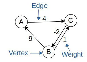
Irrespective of application, graph search algorithms are important as they let us use graphs to find optimal route, to avoid obstacles or find the degrees of separation. The relevance of graph search algorithms for graphs warrants an investment into exploration of their parallelized versions. We do an in-depth analysis of their parallelization and test our predictions using CUDA. Graph Search AlgorithmsHere I briefly explain each of the algorithms I mentioned above, derive their theoretical complexities and discuss the ways to parallelize them. Bellman-Ford AlgorithmBellman-Ford algorithm computes the shortest paths from a single-source vertex to all the other vertices in the graph. It works by going through each edge (assume edges are weighted) and updating the path to the vertex it is connected to if the current path is economical. It repeats this process |V|-1 times. It can also stop when there are no updates possible. The pseudo-code of this algorithm is shown below:
Repeat |V| - 1 times:
    For each edge e in Graph:
        if w[e.from] + w[e] < w[e.to]:
             w[e.to] = w[e.from] + w[e]
    if no updates in loop:
        return;
Typically, we also check for negative-cycles at the end of Bellman-Ford by looping one more time over all the edges. If updates are still possible then there has to be a negative weight cycle inside the graph causing the possible cost to a given edge arbitrarily low. Bellman-Ford guarantees us that if there is no negative-weight cycle present, then it converges in |V|-1 steps and gives us the optimal routes to every other vertex. Hence, it has a worst-case complexity of O(|V||E|) and a best-case time-complexity of O(|E|) in-case it converges in one outer-loop iteration. Parallelization: Now, this algorithm is easily parallelizable as the edges in the inner-loop can be explored in any order, which means we can split it into multiple threads in a GPU, which explore a subset of the edges. At the end, we synchronize the threads at the end and repeat this process |V|-1 times as before. Pseudo-code is shown below:
index = threadIdx.x + blockDim.x * blockIdx.x;
stride = blockDim.x * gridDim.x;
Repeat |V| - 1 times:
    for(e = index; i < num_edges; i+=stride):
        if w[e.from] + w[e] < w[e.to]:
            w[e.to] = w[e.from] + w[e]
    if no updates in loop:
        return;
    synchronizethreads();
Dijkstra AlgorithmWe have similar implementations of both A-Star and Dijkstra algorithms. Dijkstra can be understood as a specialized form of A-Star where the heuristic function h(x) = 0 for all x. Hence, everything in A-star algorithm section applies here with a trivial change of heuristic being zero for every input. A-Star AlgorithmA-Star algorithm is also a graph-search algorithm and can be understood as a generalized form of Dijkstra algorithm. The main difference between these two is that A-star uses a heuristic function h(x) in order to guide its search. A-star uses a priority queue and unqueues the lowest priority element at each iteration until the queue is empty or the destination is found. In this process it updates the path-costs to each vertex it encounters. A major drawback for A-Star is that it does not work for graphs with negative-weighted edges. A pseudo-code for A-star is shown below:
insert_to_queue(src, priority = 0)
while(queue not empty):
    v = dequeue();
    for each neighbour n of v:
        e = edge connecting n and v
        if w[v] + w[e] < w[n]:
            w[n] = w[v] + w[e]
        // here h[n] is the heuristic function
        if not visited:
            enqueue(n, priority = w[n] + h[n])
    if v == destination:
        return path;
The heuristic function h(x) being used in the priority in enqueueing a vertex where magic happens. If this heuristic is carefully set, then priority is given to vertices which move us towards the target node making the algorithm more efficient. Hence, A-star has a directionality in its search as opposed to Dijkstra. A very simple example of how this happens is path-finding in a map: If asked to find a route from London, UK to Bristol, UK, Dijkstra would start exploring smaller roads and highways with equal priority, but A-star would intelligently choose to explore highways first instead of wasting its time with country roads, given a sufficient heuristic. Overall, A-star has the worst-case time complexity of O(|E|) which is the same as Dijkstra's but A-star outperforms Dijkstra in practice if the heuristic is good-enough. Parallelization: We parallelized A-star algorithm using the technique described by Y. Zhao and J. Zeng in [1]. You can read the paper to get more information about the their parallelization technique. It mainly consists of having multiple queues and exploring (dequeueing) multiple nodes at the same time. Each thread is responsible for its own queue. Using thousands of queues gives the best performance which we discuss in the next section. A simple pseudo-code is given below:
initialize k queues;
insert_to_queue(queue = 0, node = src, priority = 0)
i-th thread execution:
while(all queues not empty):
    v = dequeue(queue = i);
    for each neighbour n of v:
        e = edge connecting n and v
        if w[v] + w[e] < w[n]:
            w[n] = w[v] + w[e]
    if v == destination:
        return path;
    synchronizethreads();
    deduplicate vertices already visited;
    for each neighbour n of v:
        enqueue(queue = i, node = n, priority = w[n] + h[n])
Graph API ImplementationWe implemented a very GPU-friendly graph datastructure which is inspired from adjacency list, but represents any graph using only 4 integer arrays. The 4 integer arrays are easily copied onto GPU as well and provide O(1) accesses to each vertex, edge and weight in the graph. Internally, the API uses a 0-based naming integer convention for vertices, which are also used as indices for different arrays. The representation of a simple graph is shown below to facilitate understanding: 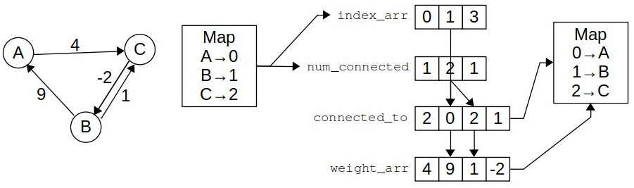
In the figure, the internal representation of the graph on the left is shown. The maps convert the vertices into 0-based indexing first. Then 4 arrays keep the track of all vertices and edges and weights. The arrows show a very simple lookup of the number of edges emanating from vertex B and their weights. In order to do that, we first convert use the mapping B→1 and consult the values of index_arr and num_connected at index 1, which are 1 and 2 respectively. 1 from index_arr tells us that edges emanating from B could be found starting at index 1 in connected_to array, while 2 from num_connected tells us that there are 2 edges emanating from B. So, we go to index 1 at both connected_to and weight_arr and look for 2 consecutive elements. connected_to tells us the ending points of those edges, which are 0 and 2, meaning A and C, while weight_arr gives us the weights of those edges: 9 and 1 respectively. Both index_arr and num_connected are of the size |V|, while connected_to and weight_arr are of the size |E|, making the total space complexity of this data-structure 2(|V|+|E|) which is way less than an adjacency matrix using |V|² space. Due to this reason, we can load up large graphs into GPU as well. Performance EvaluationFirst we examine the sequential performance of our the algorithm implementation. We plot time-taken with the number of vertices of a graph and they appear linear on a log-log scale, as the points closely follow a linear best fit. There is not much difference visible between the performance of two processors. 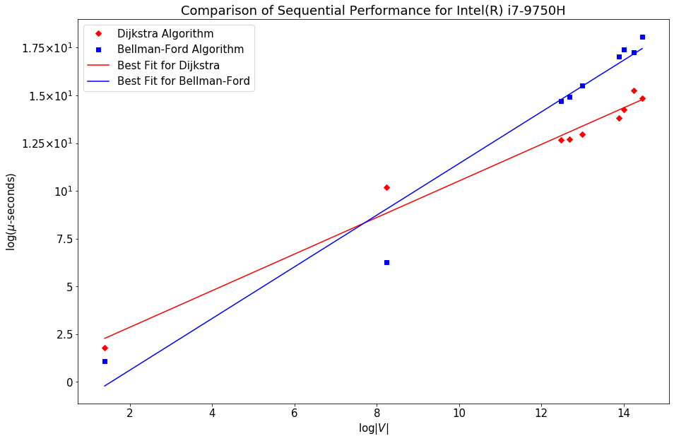
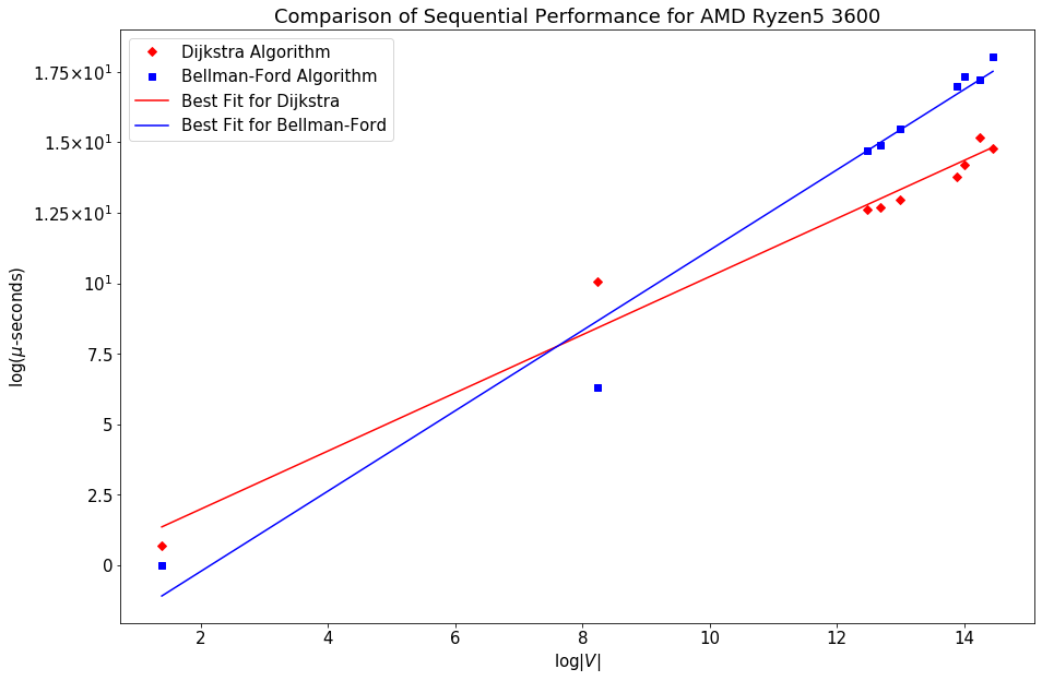
Now, we present the results for the GPU execution of these algorithms depending on the threads considered. We have used the graph with 3783 edges for this graph. Here we see that after a certain point, adding more threads for the execution does not lead to appreciable increase but on the other hand, it leads to increased overhead and may even increase the execution time. 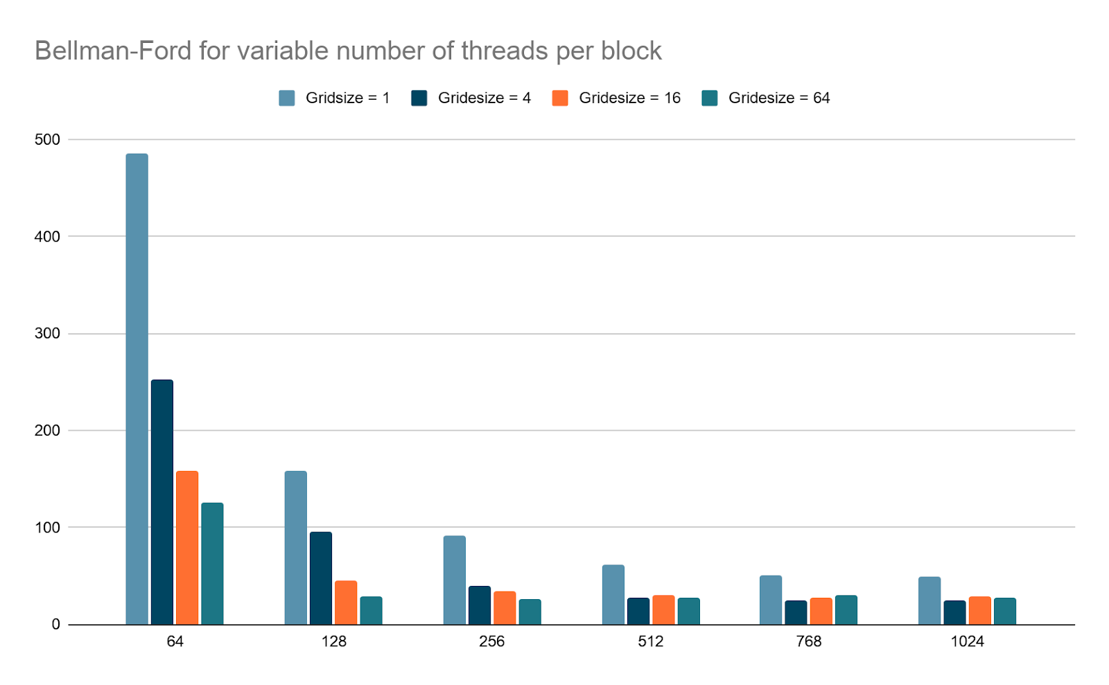
Now, we can examine the parallel performance of the Dijkstra depending on the number of parallel queues we use. The graphs are shown below and we see a similar phenomenon here that increasing the queues beyond a certain point leads to increase in execution time because of the increase in overhead. 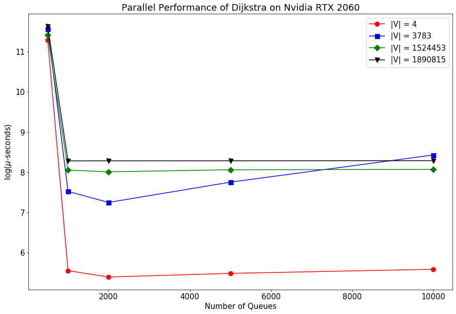
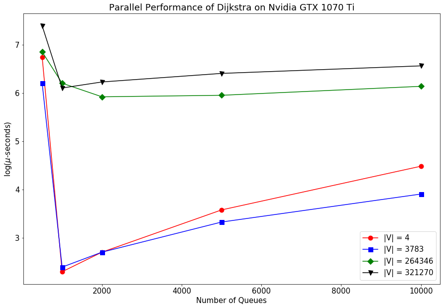
Hence, we see through these graphs that parallel computing can speed up your processes a lot but you need to be careful about the parameters you set and optimize the overhead for parallelization with the gains in execution speed. References
|